




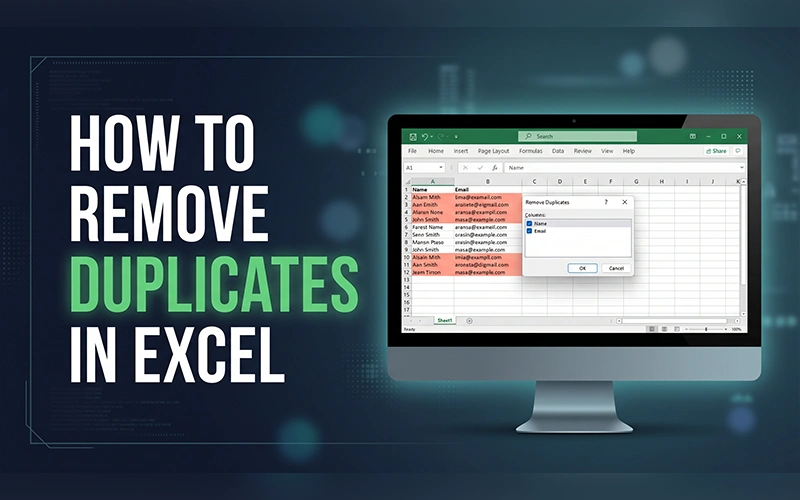
Duplicate rows rarely announce themselves. A sales total looks slightly too high, a newsletter lands twice in the same inbox, or a pivot table counts one customer as two. Learn different ways to eliminate repeated entries in Excel, from built-in features and formulas to filtering options and shortcut keys, so you can choose the method that best fits your data.
Quick answer: Select your data, open Data > Remove Duplicates, choose the columns Excel should compare, and click OK. Excel keeps the first match and deletes the later ones. Since this deletes data permanently, copy your sheet first: right-click the sheet tab, choose Move or Copy, and tick Create a copy.
Where Duplicates Come From
Most repeats sneak in through routine work. Merging exports from two systems, pasting each month’s report into one master file, importing the same CSV twice, or letting several people type into a shared sheet will all do it. Knowing the source helps you decide whether you need a one-time cleanup or a method you can repeat.
Remove Duplicates from a Single Column
Here is how to remove duplicates in Excel column A when it holds a plain list of names, SKUs, or email addresses.
- Click the column heading above the data you want to process.
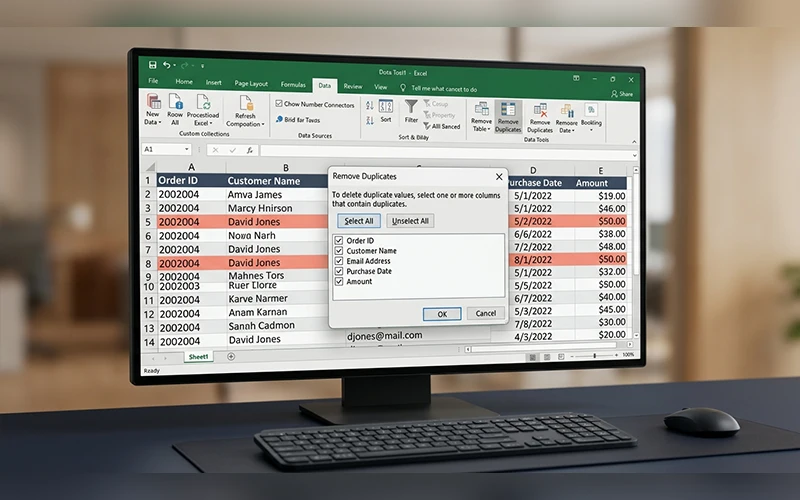
- Open the Data tab and click Remove Duplicates in the Data Tools group.
- When Excel asks about expanding the selection, choose Continue with the current selection so neighboring columns stay untouched.
- Make sure your column is ticked and click OK.
After the operation completes, Excel shows how many repeated records were deleted and how many unique entries remain in the dataset.
Keep One Copy and Delete the Rest
Most people want to know how to remove duplicates in Excel but keep one copy of each entry. The built-in tool already works this way. It scans from top to bottom, keeps the first occurrence, and deletes every later match.
This gives you control over which copy survives. Arrange the data beforehand so the record you want to retain appears first. To keep the latest entry per customer, sort by date from newest to oldest. To keep the largest order, sort by amount from high to low. Then run the tool.
Remove Duplicates Based on One Column
Two rows can share an email address yet differ in phone number or signup date, so Excel doesn’t see them as identical. That is why many users ask how to remove duplicates in Excel based on one column while ignoring the rest.
Click any cell in your table and open Data > Remove Duplicates. Click Unselect All, then tick only the column that defines a duplicate, such as Email, Employee ID, or Invoice Number. After you click OK, Excel deletes every row whose value in that column has already appeared higher up. The sorting trick from the previous section applies here too.
Clean Up an Entire Sheet
For a full worksheet, the steps are the same; only the selection changes. Click the small triangle where the row numbers meet the column letters, or click inside your table and press Ctrl + A, then open the Remove Duplicates dialog.
With every column ticked, Excel deletes a row only when all of its cells match an earlier row. That makes it the safest setting for a general cleanup, because partial matches survive.
Watch out for empty rows. Excel treats completely blank rows as duplicates of each other, so blank spacer rows between sections will collapse into one.
Remove Duplicates Without Shifting Cells
Using the built-in option deletes entire rows, shifting the remaining data upward and potentially disrupting formulas or worksheets that depend on specific cell positions. Here is how to remove duplicates in Excel without shifting cells: clear the repeated values and leave blanks in their place.
- Beside your data, enter =COUNTIF($A$2:A2,A2)>1 in the first data row, adjusting the references to your layout.
- Double-click the fill handle to copy it down. The formula returns FALSE for a first appearance and TRUE for every repeat.
- Turn on a filter from the Data tab and show only TRUE in the helper column.
- Select the visible duplicate cells in your data column and press the Delete key. Don’t use “Delete Row.”
- Clear the filter and remove the helper column.
All duplicate entries are cleared, while the remaining cells stay in their original positions.
Remove Duplicates Without Deleting Rows
If you’d rather lose nothing at all, here is how to remove duplicates in Excel without deleting rows, using Advanced Filter.
Click inside your table and go to Data > Advanced. Choose Filter the list, in-place, confirm the list range, and tick Unique records only. After you click OK, Excel hides the repeated rows, and the row numbers turn blue. Select Clear in the Sort & Filter section to reveal the rows that were hidden.
To keep a clean version somewhere else, choose Copy to another location in the same dialog and point it to an empty area. Your original table stays exactly as it was.
If you only want to review repeats, select the column and use Home > Conditional Formatting > Highlight Cells Rules > Duplicate Values. This colors every copy, including the first, so it is good for inspection but not for deciding what to delete.
Remove Duplicates Using a Formula
For anyone asking how to remove duplicates in Excel using formula logic, the UNIQUE function is the cleanest answer. It works in Excel 365, Excel 2021, and Excel for the web, and it leaves your source data untouched.
Click an empty cell, type =UNIQUE(A2:A100), and press Enter. Excel spills one copy of each value down the column, and the list updates whenever the source changes.
Unique Rows and Sorted Lists
For a multi-column table, point the function at the full range, such as =UNIQUE(A2:C100). A row counts as a repeat only when all its cells match. To arrange distinct entries alphabetically, use the SORT function together with UNIQUE: =SORT(UNIQUE(A2)).
A #NAME? error means your Excel version doesn’t support UNIQUE. In that case, use the COUNTIF helper from the earlier section or the Advanced Filter.
Use a Keyboard Shortcut
Looking for a faster way? On Windows, click a cell inside your data and press Alt, then A, then M, one key after another. The Remove Duplicates window opens instantly.
Inside the window, Alt + M toggles the headers checkbox, Alt + U unselects all columns, and Alt + A selects them all. Press Enter to confirm. Excel for Mac has no reliable default for this, so use the Data tab or assign your own shortcut in the keyboard settings.
Find Duplicates Across Multiple Columns
Sometimes one column can’t tell you whether a row repeats. Two people can share a first name, and two orders can share a date. In this case, check multiple columns together to identify rows that contain the same combination of values.
COUNTIFS handles it. With data in columns A to C, enter this in a helper column:
=IF(COUNTIFS($A$2:A2,A2,$B$2:B2,B2,$C$2:C2,C2)>1,”Duplicate”,”Unique”)
The first occurrence of each combination is labeled Unique and every repeat is labeled Duplicate, so you can filter on the label.
To highlight rows instead, select your data, choose Home > Conditional Formatting > New Rule > Use a formula, and enter =COUNTIFS($A$2:$A$100,$A2,$B$2:$B$100,$B2,$C$2:$C$100,$C2)>1. Choose a background color to highlight all rows that contain matching values across the three selected columns.
Remove Duplicates in Google Sheets
Teams that move files between both apps often search for how to remove duplicates in Excel and Google Sheets together, and the Sheets process is nearly identical. Select your range, then go to Data > Data cleanup > Remove duplicates. Tick Data has header row if it applies, choose the columns to analyze, and click Remove duplicates. Sheets keeps the first instance and tells you how many rows it dropped.
UNIQUE also works there with the same syntax. =UNIQUE(A2:C100) builds a clean list elsewhere and refreshes when the source changes.
Common Mistakes to Avoid
- Unticked header box. With “My data has headers” off, Excel includes your title row in the comparison.
- Invisible differences. “Ali Khan” and “Ali Khan ” (with a trailing space) look identical but aren’t. Run =TRIM() on messy text before cleaning.
- Ticking too few columns. Comparing only the Name column deletes two different people who share a name. Tick enough columns to define a true duplicate.
Which Method Should You Choose?
| Method | Best for | Changes original data? |
| Remove Duplicates tool | Quick permanent cleanup | Yes |
| Alt + A + M | Frequent cleanups | Yes |
| UNIQUE function | Live, always-current list | No |
| Advanced Filter | Hiding or copying unique rows | No |
| COUNTIF helper column | Clearing cells in place | Only when you delete |
| COUNTIFS check | Multi-column comparison | No |
Conclusion
The best approach depends on how you want to handle the duplicate entries. Use the built-in tool for a fast permanent cleanup, UNIQUE for reports that must stay current, and the filter or helper-column methods when your layout can’t change. Pick the one that fits, and your numbers will match reality.
Frequently Asked Questions
Can I undo Remove Duplicates?
Yes, with Ctrl + Z, but only right after running it. After you save and close the file, the deleted rows are gone.
Is Remove Duplicates case-sensitive?
No. “ABC” and “abc” are treated as the same value.
What can I use if my Excel has no UNIQUE function?
The Advanced Filter with “Unique records only” works in every version, including older ones.
Does Excel compare displayed values or stored values?
It compares what you see in the cell. Two identical dates formatted differently, such as 3/8/2026 and Mar 8, 2026, are treated as unique.
Will the remaining rows change order?
No. Excel only deletes the repeats, so the surviving rows keep their original order.
Can I check how many duplicates exist before deleting anything?
Yes. Add the COUNTIF helper column, filter it to TRUE, and read the record count in the bottom-left corner of the Excel window.
Can Remove Duplicates compare two different sheets?
No, it only works inside the selected range. To compare sheets, use a formula such as =COUNTIF(Sheet2!$A$2:$A$100,A2)>0, indicating TRUE if the same value is found in Sheet2.
Can I remove duplicates with Power Query?
Yes. Select your table, go to Data > From Table/Range, select the columns to compare, then choose Home > Remove Rows > Remove Duplicates and click Close & Load. Your source data stays untouched, and the result refreshes when the source changes.
For more articles like this, visit our site: https://factbreaker.com/